
Generate scenarios correlated to existing ones
In quantitative finance we often look at simulations of some market risk factors like equity returns or interest rate changes.
There are many third party companies who specialize in the historical calibration of such variables and provide simulations of future expected outcomes to the companies who require them.
For example, let’s suppose that we receive the expected returns of the Google shares as per the following distribution
# This modelling is given by the third party and in theory we don't know it
google <- rnorm(10000, mean = 0.01, sd = 0.20) %>%
  tibble(google_returns = .)

ggplot(data = google, aes(x = google_returns)) +
  geom_density() +
  scale_x_continuous(labels = percent) +
  labs(title = "Google Shares",
        subtitle = "One Year forward distribution") +
  xlab("One year forward return") +
  ylab("Density")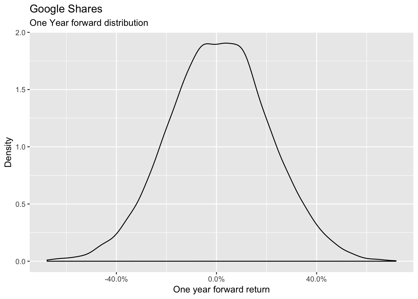
We now want to simulate the distribution of another risk factor which is not provided by the third party but that is usefull for us. Let’s say it is the distribution of the Facebook shares which we imagine to:
- be distributed as a normal random variable
- have a 5% expected return and
- being quite volatile (30% annual volatility)
- have the same number of points as the simulations provided by the third party (10000 points)
We model therefore the distribution as follows:
# This modelling is our internal one and we can therefore control it
fb <- rnorm(10000, mean = 0.05, sd = 0.30) %>%
  tibble(fb_returns = .)

ggplot(data = fb, aes(x = fb_returns)) +
  geom_density() +
  scale_x_continuous(labels = percent) +
  labs(title = "Facebook Shares",
        subtitle = "One Year forward distribution") +
  xlab("One year forward return") +
  ylab("Density")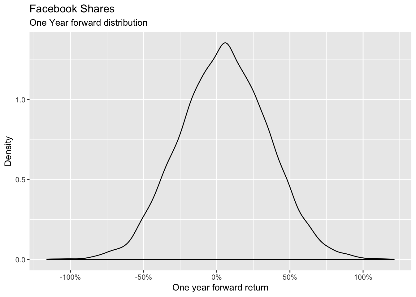
Let’s now look at the correlation between the two variables:
Returns <- google %>%
  cbind(fb) %>%
  as.tibble()
## Warning: `as.tibble()` is deprecated, use `as_tibble()` (but mind the new semantics).
## This warning is displayed once per session.cor(Returns$fb_returns, Returns$google_returns)## [1] -0.006146476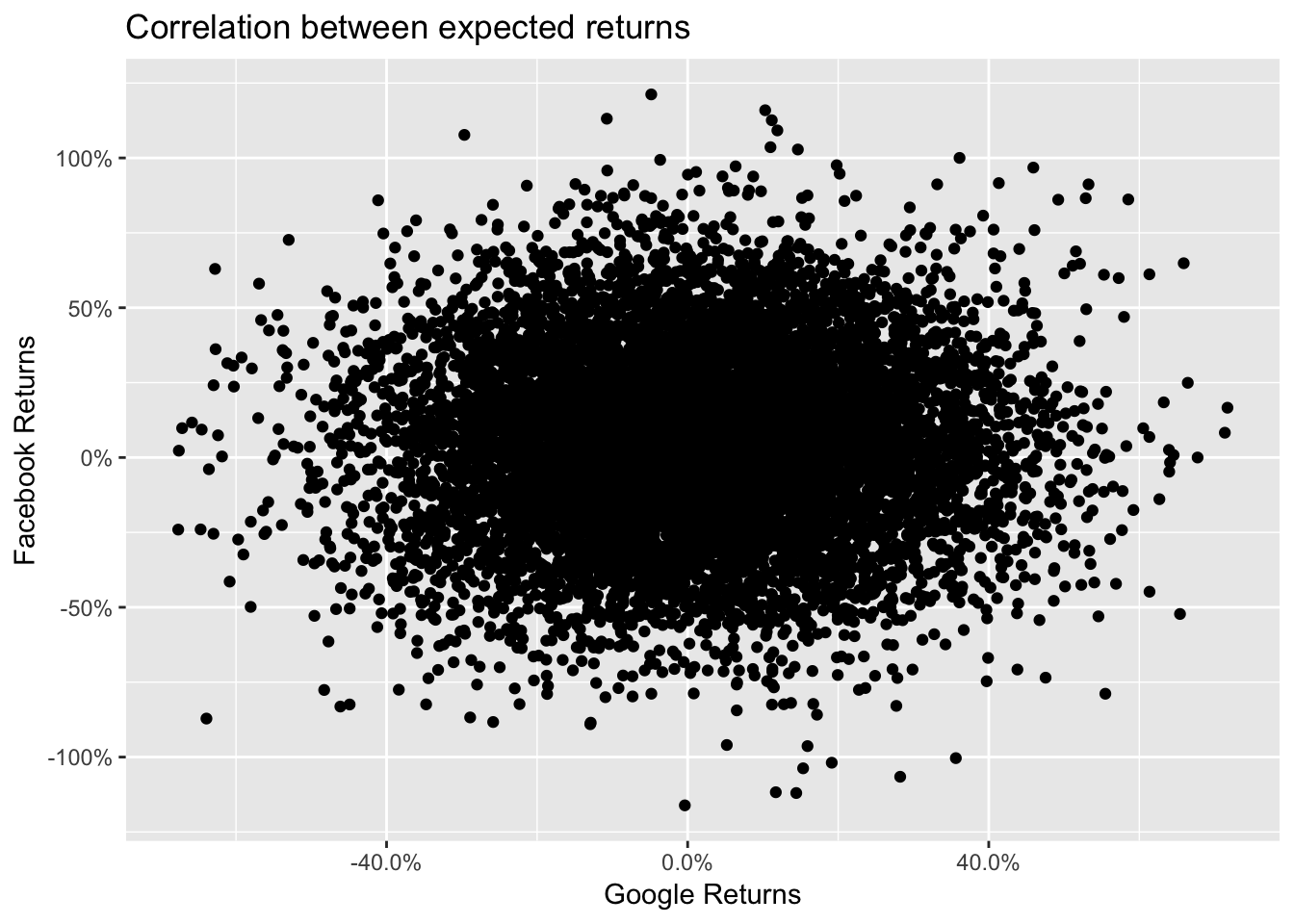
We can notice that performing the simple simulation doesn’t allow us to impose a correlation structure with the data provided by the third party provider.
How can we generate a random variable with a defined correlation to an existing one? A very elegant solution was provided by user whuber at the following link https://stats.stackexchange.com/a/313138 and by using the following function
complement <- function(y, rho, x) {
  if (missing(x)) x <- rnorm(length(y)) # Optional: supply a default if `x` is not given
  y.perp <- residuals(lm(x ~ y))
  rho * sd(y.perp) * y + y.perp * sd(y) * sqrt(1 - rho^2)
}
In this function x is our Facebook uncorrelated scenario , rho is the correlation level and y is the Google scenario as provided by the third party.
We apply this function imposing an 80% correlation
Returns %<>%
  mutate(fb_correlated = complement(.$google_returns,0.8, .$fb_returns))

cor(Returns$google_returns, Returns$fb_correlated)
## [1] 0.8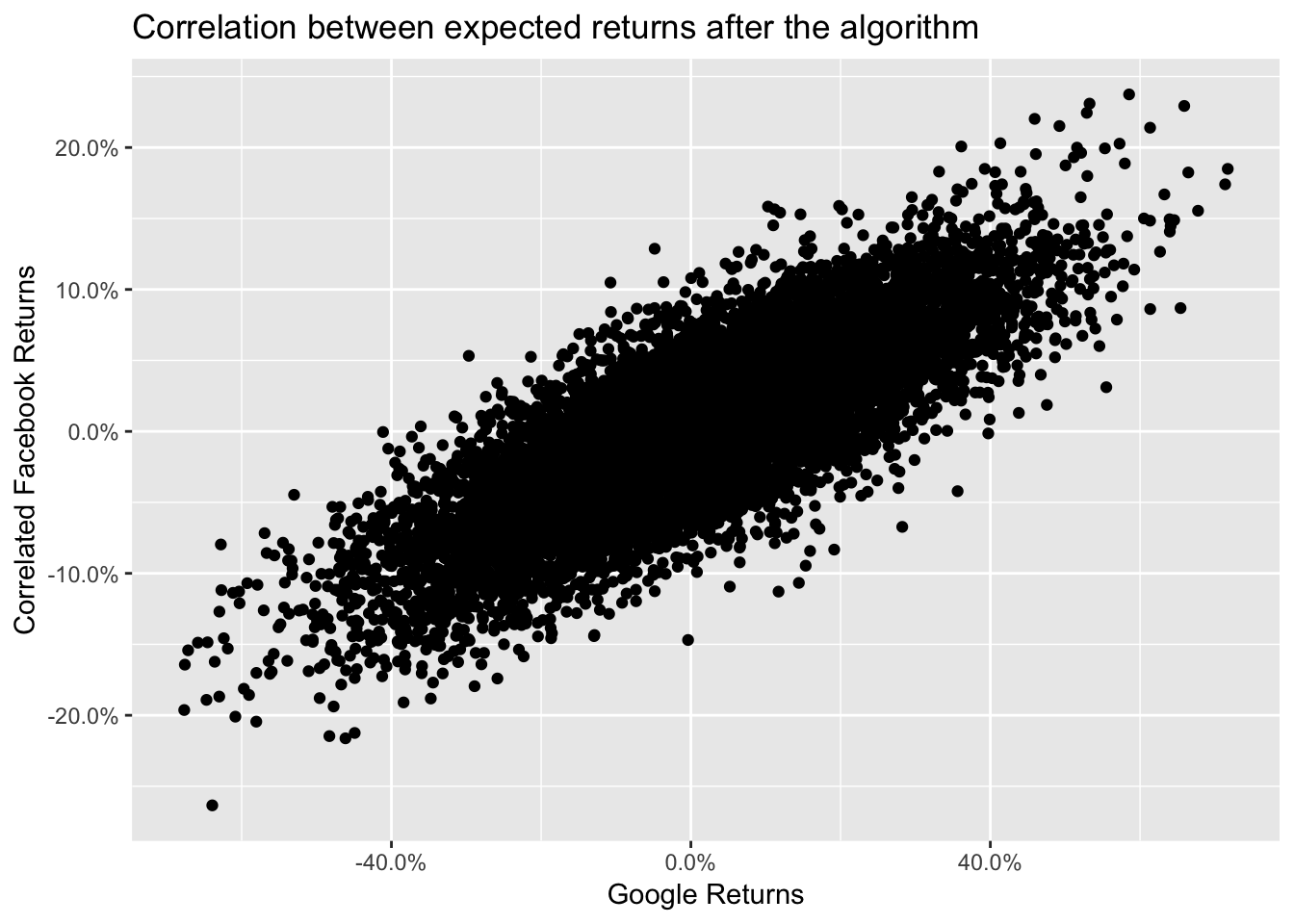
There is just one last thing to do: compare the distributions of the two Facebook simulations
Returns %>%
  select(contains("fb")) %>%
  gather(simulation_type, simulation_value) %>%
  ggplot(aes(x = simulation_value, colour = simulation_type)) +
  geom_density() +
  scale_x_continuous(labels = percent) +
  labs(title = "Facebook Shares' simulations") +
  xlab("One year forward return") +
  ylab("Density")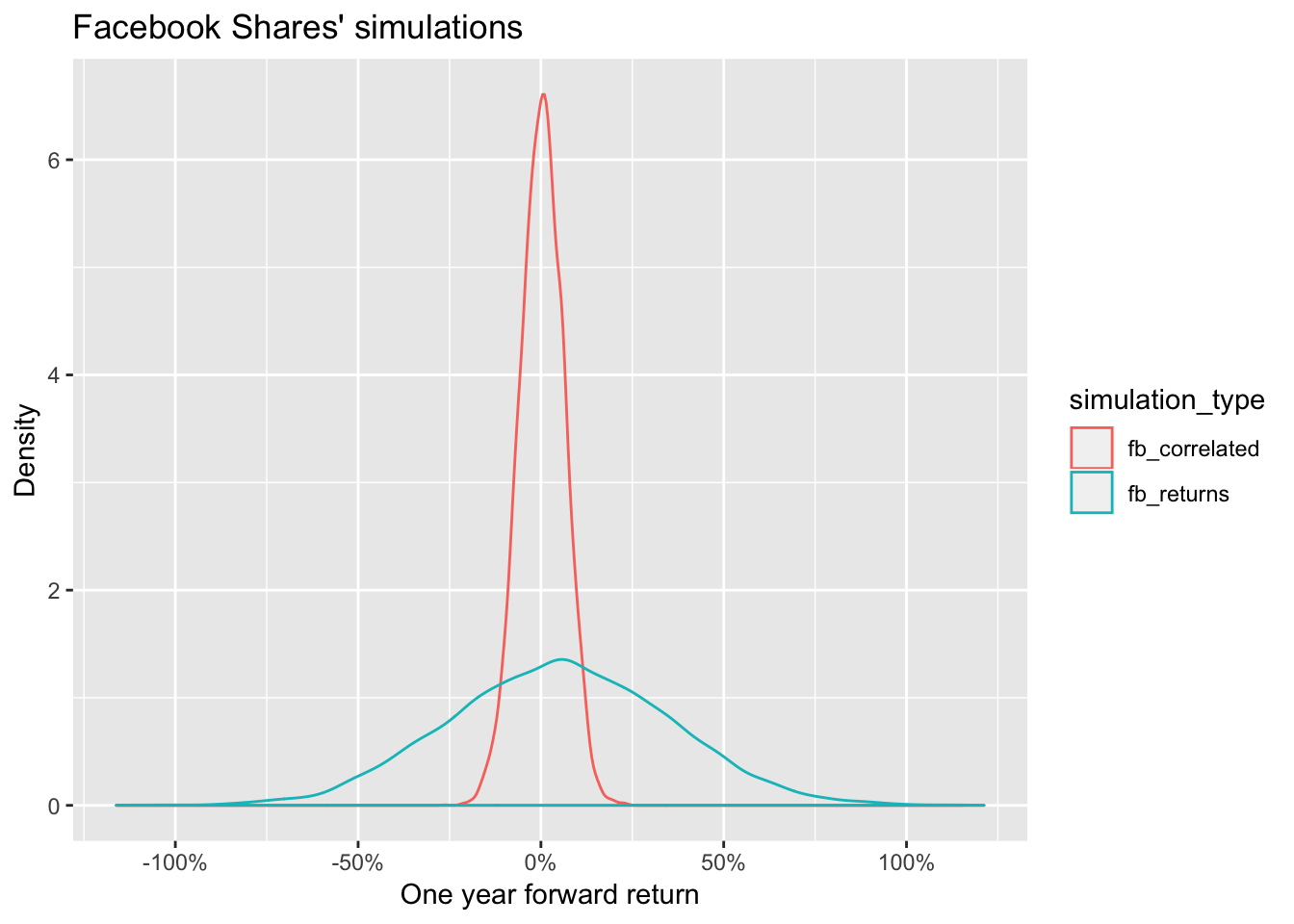
We can notice that the marginal distribution of the correlated scenario is much different from the original one.
There is therefore one additional step before we finish: we need to rescale the marginal distribution.
Rescaled_fb_correlated <- Returns %>%
  select(contains("correlated")) %>%
  scale() %>%
  multiply_by(0.3) %>%
  add(0.05)

Returns %<>%
  mutate(fb_correlated_scaled = Rescaled_fb_correlated)
We can now check that the the marginals are comparable and that the correlation structure is still at the desired level
Returns %>%
  select(contains("fb")) %>%
  gather(simulation_type, simulation_value) %>%
  ggplot(aes(x = simulation_value, colour = simulation_type)) +
  geom_density() +
  scale_x_continuous(labels = percent) +
  labs(title = "Facebook Shares' simulations") +
  xlab("One year forward return") +
  ylab("Density")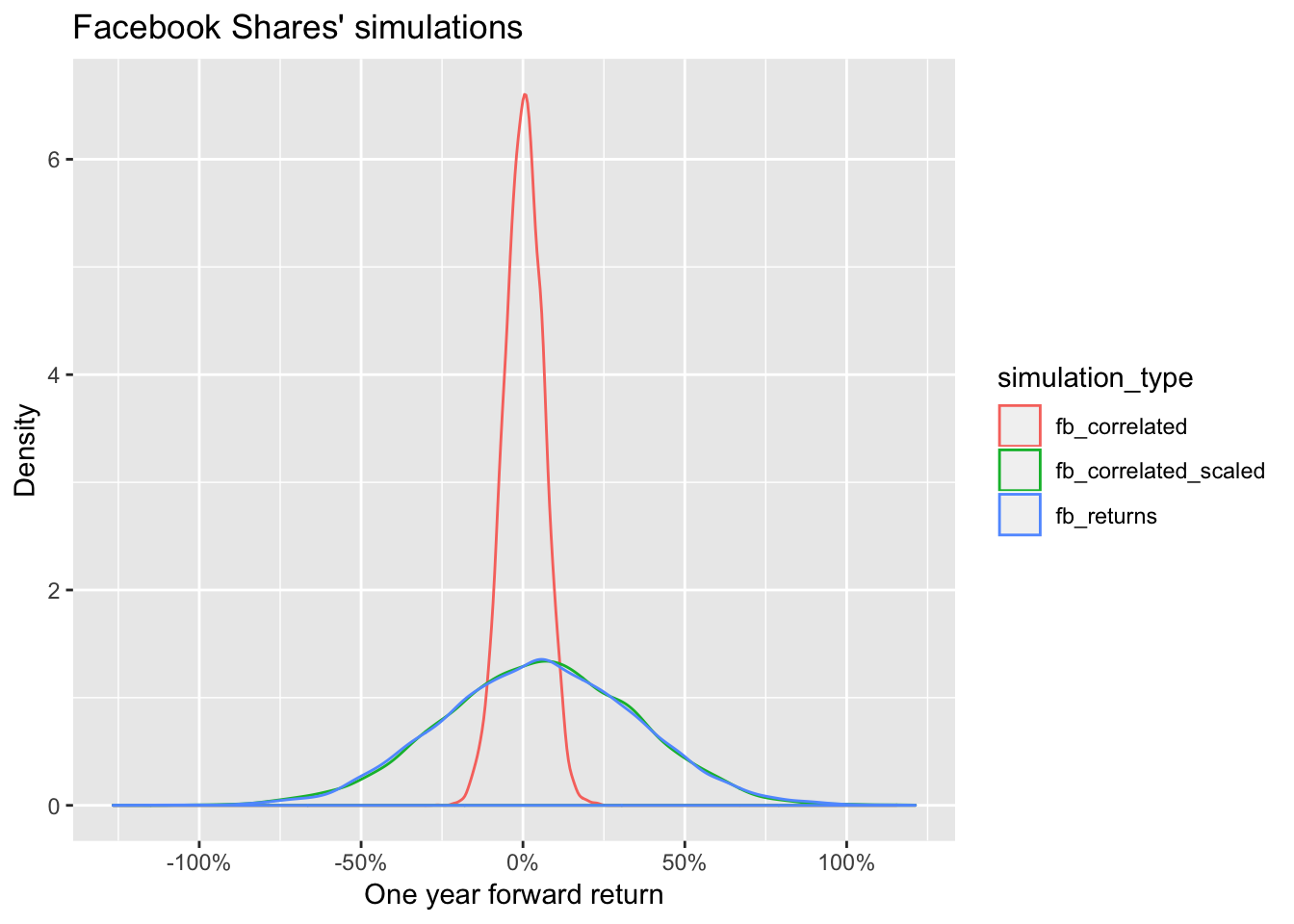
cor(Returns$google_returns, Returns$fb_correlated)## [1] 0.8The new Facebook scenario is now both correlated and in line with the density we want.

